tcal Documentation
Requirements
Python 3.11 or newer
NumPy
Gaussian 09 or 16 (optional)
PySCF (optional, macOS / Linux / WSL2(Windows Subsystem for Linux))
ORCA 6.1.0 or newer (optional)
Important
When using Gaussian, the path of the Gaussian must be set.
Important
PySCF is supported on macOS and Linux. Windows users must use WSL2.
Important
When using ORCA, ORCA must be installed. To perform parallel calculations with ORCA, OpenMPI must be configured.
Installation
Using Gaussian 09 or 16 (without PySCF)
pip install yu-tcal
Using PySCF (CPU only, macOS / Linux / WSL2)
pip install "yu-tcal[pyscf]"
Using GPU acceleration with PySCF (macOS / Linux / WSL2)
Check your installed CUDA Toolkit version:
nvcc --versionInstall tcal with GPU acceleration:
If your CUDA Toolkit version is 13.x:
pip install "yu-tcal[gpu4pyscf-cuda13]"
If your CUDA Toolkit version is 12.x:
pip install "yu-tcal[gpu4pyscf-cuda12]"
If your CUDA Toolkit version is 11.x:
pip install "yu-tcal[gpu4pyscf-cuda11]"
Using ORCA
pip install "yu-tcal[orca]"
Verify Installation
After installation, you can verify by running:
tcal --help
Options
Short |
Long |
Explanation |
|---|---|---|
|
|
Perform atomic pair transfer analysis. |
|
|
Generate cube files. |
|
|
Use Gaussian 09. (default is Gaussian 16) |
|
|
Show options description. |
|
|
Perform atomic pair transfer analysis of LUMO. |
|
|
Print MO coefficients, overlap matrix and Fock matrix. |
|
|
Output csv file on the result of apta. |
|
|
Read log/checkpoint files without executing calculations. |
|
|
Convert xyz file to gjf file. (Gaussian only) |
|
|
Calculation method and basis set in “METHOD/BASIS” format. (default: B3LYP/6-31G(d,p)) |
|
Set the number of CPUs. (default: 4) |
|
|
Set the memory size in GB. (default: 16) |
|
|
Perform atomic pair transfer analysis between different levels. N1 is the number of level in the first monomer. N2 is the number of level in the second monomer. |
|
|
Calculate the transfer integral of heterodimer. N is the number of atoms in the first monomer. |
|
|
Calculate transfer integrals between different levels. N is the number of levels from HOMO-LUMO. N=0 gives all levels. |
|
|
Skip specified calculation. If N is 1, skip 1st monomer calculation. If N is 2, skip 2nd monomer calculation. If N is 3, skip dimer calculation. |
|
|
Use PySCF instead of Gaussian. Input file must be an xyz file. |
|
|
Use GPU acceleration via gpu4pyscf. (PySCF only) |
|
|
Use Basis Set Exchange to obtain basis sets. Allows use of basis sets not included in PySCF. (PySCF only) |
|
|
Path to OpenMPI installation directory for ORCA parallel execution (sets |
How to Use
Using Gaussian
1. Create gjf file
First of all, create a gaussian input file as follows:
Example: xxx.gjf
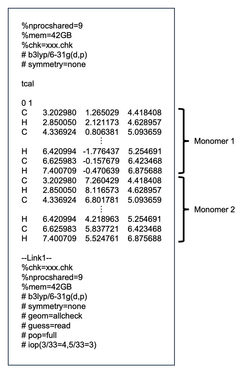
The xxx part is an arbitrary string.
Description of link commands
- pop=full
Required to output coefficients of basis functions, overlap matrix, and Fock matrix.
- iop(3/33=4,5/33=3)
Required to output coefficients of basis functions, overlap matrix, and Fock matrix.
How to create a gjf using Mercury
Open cif file in Mercury.
Display the dimer you want to calculate.
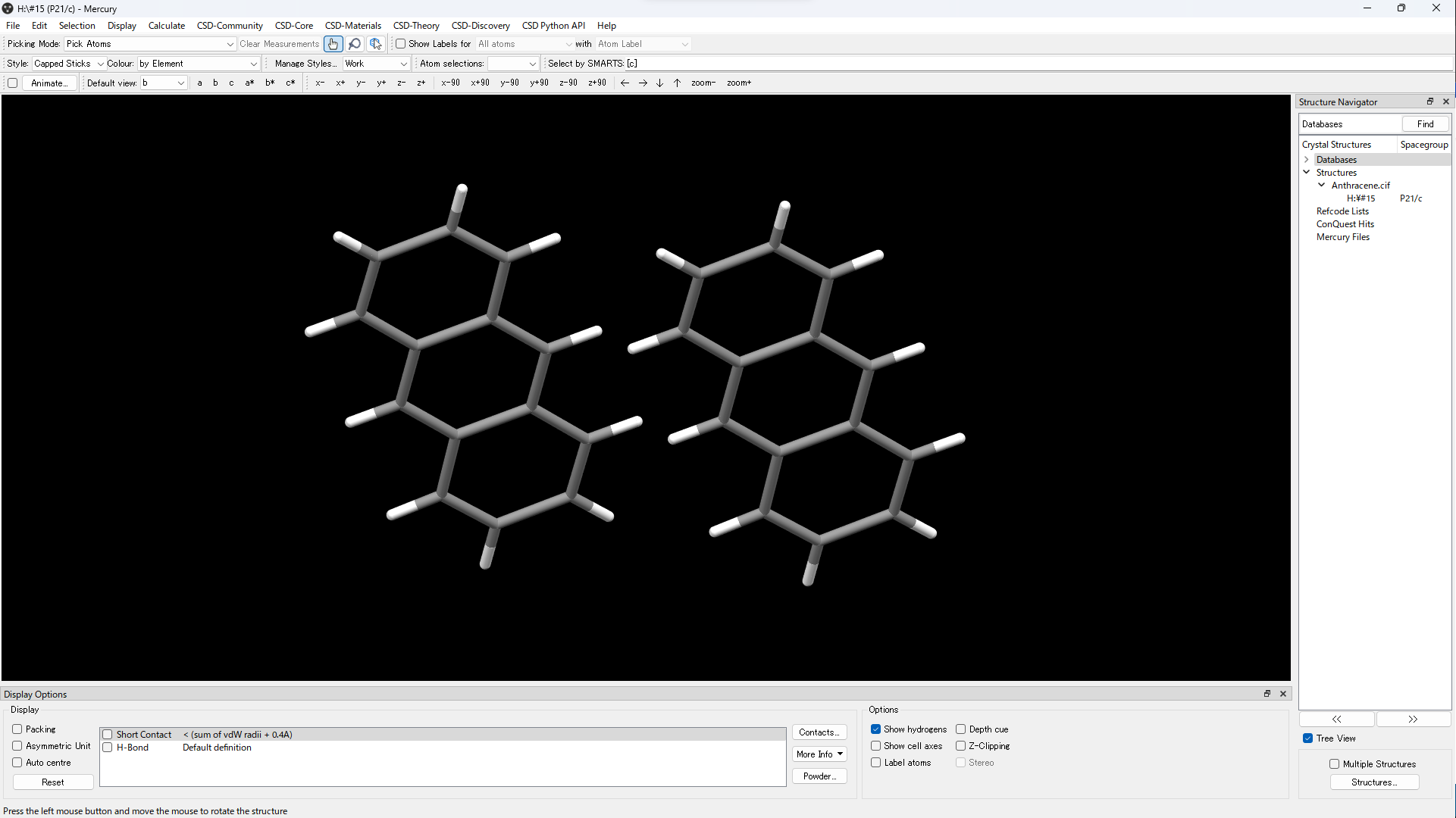
Save in mol file or mol2 file.
Open a mol file or mol2 file in GaussView and save it in gjf format.
2. Execute tcal
Suppose the directory structure is as follows:
yyy
└── xxx.gjf
Open a terminal.
Go to the directory where the files is located.
cd yyy
Execute the following command.
tcal -a xxx.gjf
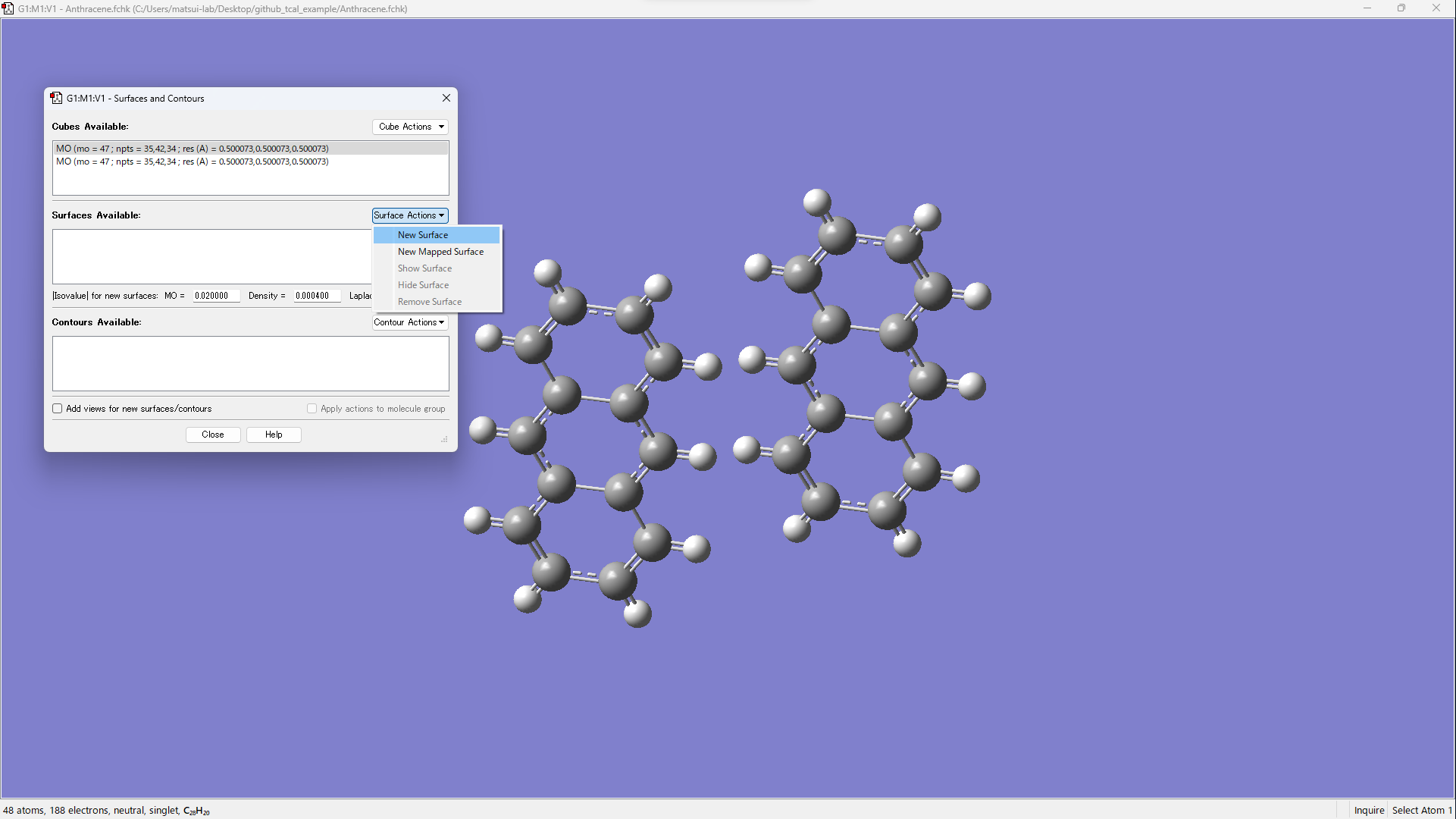
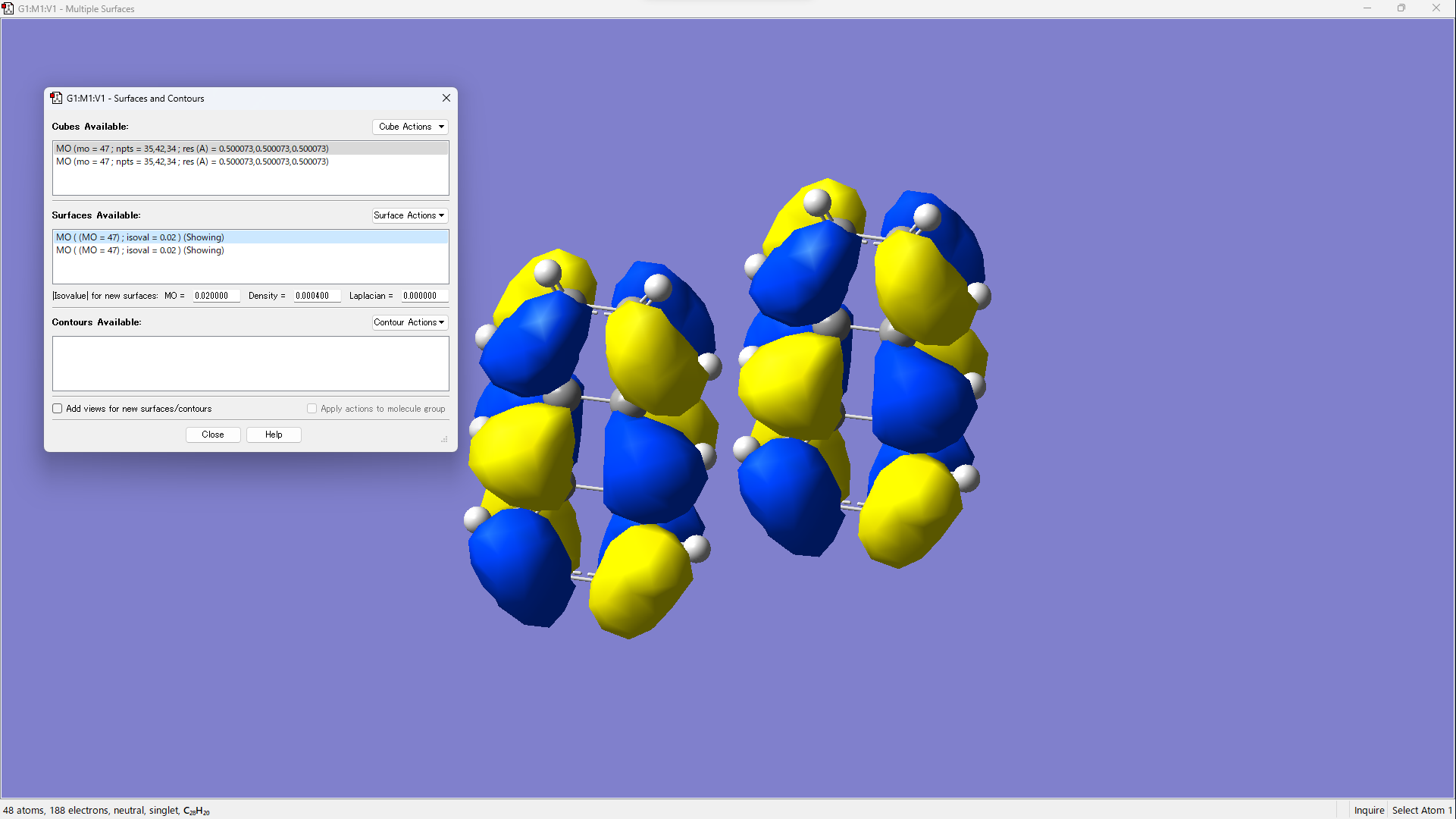
3. Visualization of molecular orbitals
Execute the following command.
tcal -cr xxx.gjf
Open xxx.fchk in GaussView.
[Results] → [Surfaces/Contours…]
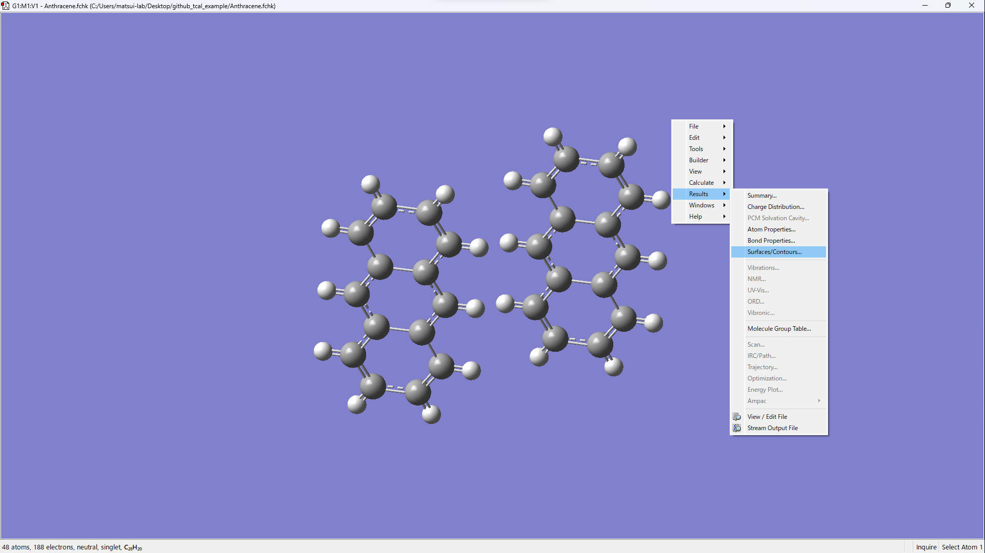
[Cube Actions] → [Load Cube]
Open xxx_m1_HOMO.cube and xxx_m2_HOMO.cube.
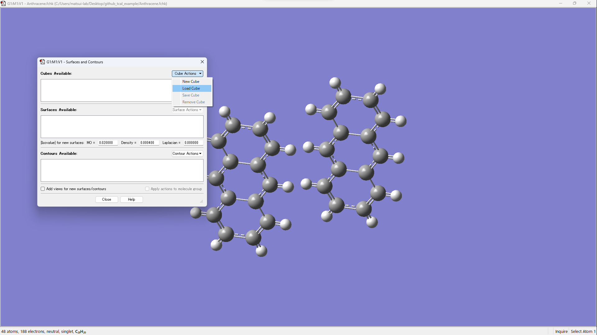
Visualize by operating [Surface Actions] → [New Surface].
Using PySCF
1. Create xyz file
Prepare an xyz file of the dimer structure.
The first half of the atoms are treated as monomer 1, and the second half as monomer 2.
For heterodimers, use the --hetero N option to specify the number of atoms in the first monomer.
2. Execute tcal
tcal --pyscf -a xxx.xyz
To specify a calculation method and basis set:
tcal --pyscf -M "B3LYP/6-31G(d,p)" -a xxx.xyz
To use GPU acceleration:
tcal --gpu4pyscf -M "B3LYP/6-31G(d,p)" -a xxx.xyz
To use basis sets from Basis Set Exchange (e.g., def2-TZVP, cc-pVDZ):
tcal --pyscf --bse -M "B3LYP/def2-TZVP" -a xxx.xyz
To read from existing checkpoint files without re-running calculations:
tcal --pyscf -ar xxx.xyz
Using ORCA
1. Create xyz file
Prepare an xyz file of the dimer structure.
The first half of the atoms are treated as monomer 1, and the second half as monomer 2.
For heterodimers, use the --hetero N option to specify the number of atoms in the first monomer.
2. Execute tcal
tcal --orca -a xxx.xyz
To specify a calculation method and basis set:
tcal --orca -M "B3LYP/6-31G(d,p)" -a xxx.xyz
To read from existing output files without re-running calculations:
tcal --orca -ar xxx.xyz
3. Parallel execution
To use multiple CPU cores (--cpu N), OpenMPI must be installed.
First, confirm that mpirun is available:
which mpirun
If OpenMPI is already in $PATH and $LD_LIBRARY_PATH (common on Linux/WSL after apt install), no further configuration is needed.
If parallel execution does not work, find the OpenMPI base directory (the directory that contains bin/ and lib/) and pass it via OPI_MPI or --mpi.
Linux / WSL
Important
ORCA requires a specific version of OpenMPI. The version available via apt may not match.
If parallel execution fails, it is recommended to build OpenMPI from source using the version
specified in the ORCA documentation.
When mpirun is installed under a dedicated directory (e.g., built from source or via a module system):
which mpirun
# e.g., /opt/openmpi/bin/mpirun  →  base: /opt/openmpi
export OPI_MPI=$(dirname $(dirname $(which mpirun)))
When installed system-wide via apt (Ubuntu/Debian), mpirun is typically at /usr/bin/mpirun
but the OpenMPI libraries live under /usr/lib/. Check with:
which mpirun
# /usr/bin/mpirun  →  base is usually /usr/lib/x86_64-linux-gnu/openmpi
export OPI_MPI=/usr/lib/x86_64-linux-gnu/openmpi
macOS (Homebrew)
which mpirun
# e.g., /opt/homebrew/bin/mpirun
export OPI_MPI=$(brew --prefix open-mpi)
Passing the path with --mpi
Instead of setting the environment variable, you can pass the path directly:
tcal --orca --cpu 8 --mpi /path/to/openmpi -a xxx.xyz
Interatomic Transfer Integral
For calculating the transfer integral between molecule A and molecule B, DFT calculations were performed for monomer A, monomer B, and the dimer AB. The monomer molecular orbitals \(\ket{A}\) and \(\ket{B}\) were obtained from the monomer calculations. Fock matrix F was calculated in the dimer system. Finally the intermolecular transfer integral \(t^{[1]}\) was calculated by using the following equation:
where \(\epsilon_A \equiv \braket{A|F|A}\) and \(\epsilon_B \equiv \braket{B|F|B}\).
In addition to the intermolecular transfer integral in general use, we developed an interatomic transfer integral for further analysis \(^{[2]}\). By grouping the basis functions \(\ket{i}\) and \(\ket{j}\) for each atom, the molecular orbitals can be expressed as
where \(\alpha\) and \(\beta\) are the indices of atoms, \(i\) and \(j\) are indices of basis functions, and \(a_i\) and \(b_j\) are the coefficients of basis functions. Substituting this formula into aforementioned equation gives
Here we define the interatomic transfer integral \(u_{\alpha\beta}\) as:
References
[1] Veaceslav Coropceanu et al., Charge Transport in Organic Semiconductors, Chem. Rev. 2007, 107, 926-952.
[2] Koki Ozawa et al., Statistical analysis of interatomic transfer integrals for exploring high-mobility organic semiconductors, Sci. Technol. Adv. Mater. 2024, 25, 2354652.
[3] Qiming Sun et al., Recent developments in the PySCF program package, J. Chem. Phys. 2020, 153, 024109.
[4] Benjamin P. Pritchard et al., New Basis Set Exchange: An Open, Up-to-Date Resource for the Molecular Sciences Community, J. Chem. Inf. Model. 2019, 59, 4814-4820.
[5] Frank Neese, The ORCA program system, Wiley Interdiscip. Rev. Comput. Mol. Sci., 2012, 2, 73-78.
Citation
When publishing works that benefited from tcal, please cite the following article:
Koki Ozawa, Tomoharu Okada, Hiroyuki Matsui, Statistical analysis of interatomic transfer integrals for exploring high-mobility organic semiconductors, Sci. Technol. Adv. Mater., 2024, 25, 2354652.
Example of using tcal
API Reference
API Reference
Indices and Tables
Acknowledgements
This work was supported by JST, CREST, Grand Number JPMJCR18J2.
License
This project is released under the MIT License.
For more details, see the LICENSE file on GitHub.